2.3: Applications and Modeling with Sinusoidal Functions

Ted Sundstrom & Steven Schlicker
Grand Valley State University via ScholarWorks @Grand Valley State University

What does frequency mean?
How do we model periodic data accurately with a sinusoidal function?
What is a mathematical model?
Why is it reasonable to use a sinusoidal function to model periodic phenomena?

In Section 2.2, we used the diagram in Figure $\PageIndex$ to help remember important facts about sinusoidal functions.

$2.19.png$

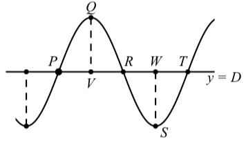
Figure $\PageIndex$: Graph of a Sinusoid

The horizontal distance between a point where a maximum occurs and the next point where a minimum occurs (such as points $Q$ and $S$) is one-half of a period. This is the length of the segment from $V$ to $W$ in Figure $\PageIndex$.
The vertical distance between a point where a minimum occurs (such as point $S$) and a point where is maximum occurs (such as point $Q$) is equal to two times the amplitude.
The center line $y = D$ for the sinusoid is half-way between the maximum value at point $Q$ and the minimum value at point $S$. The value of $D$ can be found by calculating the average of the $y$-coordinates of these two points.
The horizontal distance between any two successive points on the line $y = D$ in Figure $\PageIndex$ is one-quarter of a period.

In Progress Check 2.16, we will use some of these facts to help determine an equation that will model the volume of blood in a person’s heart as a function of time. A mathematical model is a function that describes some phenomenon. For objects that exhibit periodic behavior, a sinusoidal function can be used as a model since these functions are periodic. However, the concept of frequency is used in some applications of periodic phenomena instead of the period.

The frequency of a sinusoidal function is the number of periods (or cycles) per unit time.

A typical unit for frequency is the hertz. One hertz (Hz) is one cycle per second. This unit is named after Heinrich Hertz (1857 – 1894).

Since frequency is the number of cycles per unit time, and the period is the amount of time to complete one cycle, we see that frequency and period are related as follows:

The volume of the average heart is 140 milliliters (ml), and it pushes out about one-half its volume (70 ml) with each beat. In addition, the frequency of the for a well-trained athlete heartbeat for a well-trained athlete is 50 beats (cycles) per minute. We will model the volume, V .t / (in milliliters) of blood in the heart as a function of time t measured in seconds. We will use a sinusoidal function of the form \[V(t) = A\cos(B(t - C)) + D\]

If we choose time 0 minutes to be a time when the volume of blood in the heart is the maximum (the heart is full of blood), then it reasonable to use a cosine function for our model since the cosine function reaches a maximum value when its input is 0 and so we can use $C = 0$, which corresponds to a phase shift of 0. So our function can be written as $V(t) = A\cos(Bt) + D$.

What is the maximum value of $V(t)$? What is the minimum value of $V(t)$? Use these values to determine the values of $A$ and $D$ for our model? Explain.
Since the frequency of heart beats is 50 beats per minute, we know that the time for one heartbeat will be 1 of a minute. Determine the time (in 50 seconds) it takes to complete one heartbeat (cycle). This is the period for this sinusoidal function. Use this period to determine the value of B. Write the formula for $V(t)$ using the values of $A, B, C$, and $D$ that have been determined.

The maximum value of $V(t)$ is $140$ ml and the minimum value of $V(t)$ is $70$ ml. So the difference $(140 - 70 = 70)$ is twice the amplitude. Hence, the amplitude is $35$ and we will use $A = 35$. The center line will then be $35$ units below the maximum. That is, $D = 140 - 35 = 105$.

Since there are $50$ beats per minute, the period is $\dfrac$ of a minute. Since we are using seconds for time, the period is $\dfrac$ seconds or $\dfrac$ sec. We can determine $B$ by solving the equation \[\dfrac<2\pi> = \dfrac\] for $B$. This gives $B = \dfrac<10\pi> = \dfrac<5\pi>$. Our function is

(Continuation of Progress Check 2.16)

Now that we have determined that \[V(t) = 35\cos(\dfrac<5\pi>t) + 105\]

(where $t$ is measured in seconds since the heart was full and $V(t)$ is measured in milliliters) is a model for the amount of blood in the heart, we can use this model to determine other values associated with the amount of blood in the heart. For example:

We can determine the amount of blood in the heart $1$ second after the heart was full by using $t = 1$. \[V(1) = 35\cos(\dfrac<5\pi>) + 105\] So we can say that $1$ second after the heart is full, there will be $122.5$ milliliters of blood in the heart.

In a similar manner, $4$ seconds after the heart is full of blood, there will be $87.5$ milliliters of blood in the heart since \[V(4) = 35\cos(\dfrac<20\pi>) + 105 \approx 87.5\]

Suppose that we want to know at what times after the heart is full that there will be 100 milliliters of blood in the heart. We can determine this if we can solve the equation $V(t) = 100$ for $t$. That is, we need to solve the equation \[35\cos(\dfrac<5\pi>t) + 105 = 100\]

Although we will learn other methods for solving this type of equation later in the book, we can use a graphing utility to determine approximate solutions for this equation. Figure $\PageIndex$ shows the graphs of $y = V(t)$ and $y = 100$. To solve the equation, we need to use a graphing utility that allows us to determine or approximate the points of intersection of two graphs. (This can be done using most Texas Instruments calculators and Geogebra.) The idea is to find the coordinates of the points $P, Q$, and $R$ in Figure $\PageIndex$.

$2.20.png$

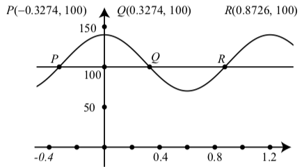
Figure $\PageIndex$: Graph of $V(t) = 35\cos(\dfrac<5\pi>) + 105$ and $y = 100$

We really only need to find the coordinates of one of those points since we can use properties of sinusoids to find the others. For example, we can determine that the coordinates of $P$ are $(-0.3274, 100)$. Then using the fact that the graph of $y = V(t)$ is symmetric about the y-axis, we know the co- ordinates of $Q$ are $(0.3274, 100)$. We can then use the periodic property of the function, to determine the $t$-coordinate of $R$ by adding one period to the $t$-coordinate of $P$. This gives $0.3274 + \dfrac = 0.8726$, and the coordinates of $R$ are $(0.8726, 100)$. We can also use the periodic property to determine as many solutions of the equation $V(t) = 100$ as we like.

The summer solstice in 2014 was on June 21 and the winter solstice was on December 21. The maximum hours of daylight occurs on the summer solstice and the minimum hours of daylight occurs on the winter solstice. According to the U.S. Naval Observatory website, aa.usno.navy.mil/data/docs/Dur_OneYear.php,

the number of hours of daylight in Grand Rapids, Michigan on June 21, 2014 was 15.35 hours, and the number of hours of daylight on December 21, 2014 was 9.02 hours. This means that in Grand Rapids,

The maximum number of hours of daylight was $15.35$ hours and occurred on day $172$ of the year.
The minimum number of hours of daylight was $9.02$ hours and occurred on day $355$ of the year.

1. Let $y$ be the number of hours of daylight in 2014 in Grand Rapids and let $t$ be the day of the year. Determine a sinusoidal model for the number of hours of daylight $y$ in 2014 in Grand Rapids as a function of $t$.

2. According to this model,

(a) How many hours of daylight were there on March 10, 2014?
(b) On what days of the year were there 13 hours of daylight?

1. Since we have the coordinates for a high and low point, we first do the following computations:

$2(amp) = 15.35 - 9.02 = 6.33$. Hence, the amplitude is $3.165$.

\[D = 9.02 + 3.165 = 12.185\].

$\dfrac$ period $= 355 - 172 = 183$. So the period is $366$. Please note that we usually say that there are $365$ days in a year. So it would also be reasonable to use a period of $365$ days. Using a period of $366$ days, we find that \[\dfrac<2\pi> = 366\]

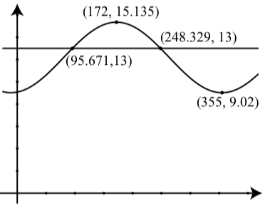
We must now decide whether to use a sine function or a cosine function to get the phase shift. Since we have the coordinates of a high point, we will use a cosine function. For this, the phase shift will be 172. So our function is

\[y = 3.165\cos(\dfrac<\pi>(t - 172)) + 12.185\]

We can check this by verifying that when $t = 155, y = 15.135$ and that when $t = 355, y = 9.02$.

(a) March $10$ is day number $69$. So we use $t = 69$ and get \[y = 3.165\cos(\dfrac<\pi>(69 - 172)) + 12.185 \approx 11.5642\]

So on March 10, 2014, there were about $11.564$ hours of daylight.

(b) We use a graphing utility to approximate the points of intersection of $y = 3.165\cos(\dfrac<\pi>(69 - 172)) + 12.125$ and $y = 13$. The results are shown to the right. So on day 96 (April 6, 2014) and on day 248 (September 5), there were about 13 hours of daylight.

$pc 2.18.png$

Determining a Sinusoid from Data

In Progress Check 2.18 the values and times for the maximum and minimum hours of daylight. Even if we know some phenomenon is periodic, we may not know the values of the maximum and minimum. For example, the following table shows the number of daylight hours (rounded to the nearest hundredth of an hour) on the first of the month for Edinburgh, Scotland $(55^\circ 57' N, 3^\circ 12' W)$.

We will use a sinusoidal function of the form $y = A\sin(B(t - C)) + D$, where $y$ is the number of hours of daylight and $t$ is the time measured in months to model this data. We will use 1 for Jan., 2 for Feb., etc. As a first attempt, we will use $17.48$ for the maximum hours of daylight and $7.08$ for the minimum hours of daylight.

Jan	Feb	Mar	Apr	May	June	July	Aug	Sept	Oct	Nov	Dec
7.08	8.60	10.73	13.15	15.40	17.22	17.48	16.03	13.82	11.52	9.18	7.40

Table 2.2: Hours of Daylight in Edinburgh

Since $17.48 - 7.08 = 10.4$, we see that the amplitude is 5.2 and so $A = 5.2$.
The vertical shift will be $7.08 + 5.2 = 12.28$ and so $D = 12.28$.
The period is 12 months and so $B = \dfrac<2\pi>= \dfrac<\pi>$.
The maximum occurs at $t = 7$. For a sine function, the maximum is one- quarter of a period from the time when the sine function crosses its horizontal axis. This indicates a phase shift of 4 to the right. So $C = 4$.

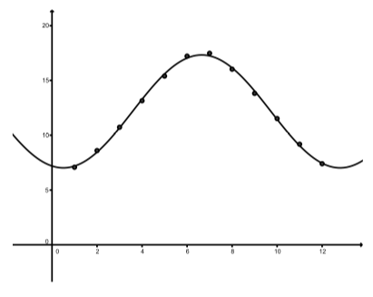
So we will use the function $y = 5.2\sin(\dfrac<\pi>(t - 4)) + 12.28$ to model the number of hours of daylight. Figure $\PageIndex$ shows a scatter plot for the data and a graph of this function. Although the graph fits the data reasonably well, it seems we should be able to find a better model. One of the problems is that the maximum number of hours of daylight does not occur on July 1. It probably occurs about 10 days earlier. The minimum also does not occur on January 1 and is probably somewhat less that 7.08 hours. So we will try a maximum of 17.50 hours and a minimum of 7.06 hours. Also, instead of having the maximum occur at $t = 7$, we will say it occurs at t D 6:7. Using these values, we have $A = 5.22, B = \dfrac<\pi>, C = 3.7, \space and \space D = 12.28$. Figure 2.22 shows a scatter plot of the data and a graph of \[y = 5.22\sin(\dfrac<\pi>(t - 3.7)) + 12.28\]

This appears to model the data very well. One important thing to note is that when trying to determine a sinusoid that “fits” or models actual data, there is no single correct answer. We often have to find one model and then use our judgment in order to determine a better model. There is a mathematical “best fit” equation for a sinusoid that is called the sine regression equation. Please note that we need to use some graphing utility or software in order to obtain a sine regression equation. Many Texas Instruments calculators have such a feature as does the software Geogebra. Following is a sine regression equation for the number of hours of daylight in Edinburgh shown in Table 2.2 obtained from Geogebra.

\[y = 5.153\sin(0.511t - 1.829) + 12.174\]

A scatter plot with a graph of this function is shown in Figure $\PageIndex$.

$2.21.png$

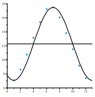
Figure $\PageIndex$: Hours of Daylight in Edinburgh

See the supplements at the end of this section for instructions on how to use Geogebra and a Texas Instruments TI-84 to determine a sine regression equation for a given set of data.

It is interesting to compare equation (1) and equation (2), both of which are models for the data in Table 2.2. We can see that both equations have a similar amplitude and similar vertical shift, but notice that equation (2) is not in our standard form for the equation of a sinusoid. So we cannot immediately tell what that equation is saying about the period and the phase shift. In this next activity, we will learn how to determine the period and phase shift for sinusoids whose equations are of the form $y = a\sin(bt + c) + d$ or $y = a\cos(bt + c) + d$.

Activity 2.19 (Working with Sinusoids that Are Not In Standard Form)

So far, we have been working with sinusoids whose equations are of the form $y = A\sin(B(t - C)) + D$ or $y = A\cos(B(t - C)) + D$. When written in this form, we can use the values of $A, B, C$, and $D$ to determine the amplitude,

$2.22.png$

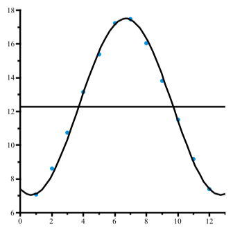
Figure $\PageIndex$: Hours of Daylight in Edinburgh

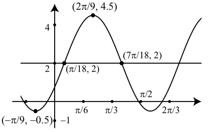
period, phase shift, and vertical shift of the sinusoid. We must always remember, however, that to to this, the equation must be written in exactly this form. If we have an equation in a slightly different form, we have to determine if there is a way to use algebra to rewrite the equation in the form $y = A\sin(B(t - C)) + D$ or $y = A\cos(B(t - C)) + D$. Consider the equation $y = 2\sin(3t + \dfrac<\pi>)$

$2.23.png$

Use a graphing utility to draw the graph of this equation with $-\dfrac<\pi>\leq t \leq \dfrac<2\pi>$and. Does this seem to be the graph of a sinusoid? If so, can you use the graph to find its amplitude, period, phase shift, and vertical shift?
It is possible to verify any observations that were made by using a little algebra to write this equation in the form $y = A\sin(B(t - C)) + D$. The idea is to rewrite the argument of the sine function, which is $3t + \dfrac<\pi>$ by “factoring a 3” from both terms. This may seem a bit strange since we are not used to using fractions when we factor. For example, it is quite easy to factor $3y + 12$ as \[3y + 12 = 3(y + 4)\]
In order to “factor” three from $\dfrac<\pi>$, we basically use the fact that $3 \cdot \dfrac= 1$ Figure $\PageIndex$: Hours of Daylight in Edinburgh So we can write \[\dfrac<\pi>= 3 \cdot \dfrac\cdot \dfrac<\pi>= 3 \cdot \dfrac<\pi>\] Now rewrite $3t + \dfrac<\pi>$ by factoring a 3 and then rewrite $y = 2\sin(3t + \dfrac<\pi>)$ in the form $y = A\sin(B(t - C)) + D$. 3. What is the amplitude, period, phase shift, and vertical shift for $y = 2\sin(3t + \dfrac<\pi>)$? In Activity 2.19, we did a little factoring to show that \[y = 2\sin(3t + \dfrac<\pi>) = 2\sin(3(t + \dfrac<\pi>))\] \[y = 2\sin(3(t - (-\dfrac<\pi>)))\] So we can see that we have a sinusoidal function and that the amplitude is 3, the period is 2, the phase shift is $\dfrac<2\pi>$, and the vertical shift is 0.
In general, we can see that if $b$ and $c$ are real numbers, then \[bt + c = b(t + \dfrac) = b(t - (-\dfrac))\] This means that \[y = a\sin(bt + c) + d = a\sin(b(t - (-\dfrac))) + d\] So we have the following result: If $y = a\sin(bt + c) + d$ or $y = a\cos(bt + c) + d$, then
The amplitude of the sinusoid is $|a|$.
The period of the sinusoid is $\dfrac<2\pi>$
The phase shift of the sinusoid is $-\dfrac$
The vertical shift of the sinusoid is $d$.

Determine the amplitude, period, phase shift, and vertical shift for each of the following sinusoids. Then use this information to graph one complete period of the sinusoid and state the coordinates of a high point, a low point, and a point where the sinusoid crosses the center line. (a) $y = -2.5\cos(3x + \dfrac<\pi>) + 2$ (b) $y = 4\sin(100\pi x - \dfrac<\pi>)$
We determined two sinusoidal models for the number of hours of daylight in Edinburgh, Scotland shown in Table 2.2. These were \[y = 5.22\sin(\dfrac<\pi>(t - 3.7)) + 12.28\] \[y = 5.153\sin(0.511t - 1.829) + 12.174\]
The second equation was determined using a sine regression feature on a graphing utility. Compare the amplitudes, periods, phase shifts, and vertical shifts of these two sinusoidal functions.

1. (a) The amplitude is $2.5$.

The period is $\dfrac<2\pi>$.

The phase shift is $-\dfrac<\pi>$. The vertical shift is $2$.

$pc 2.20 a.png$

(b) The amplitude is $4$.

The period is $\dfrac$

The phase shift is $\dfrac$.

The vertical shift is $0$.